Linear Regression
Linear regression is a linear approach to modeling the relationship between a scalar response (or dependent variable) and one or more explanatory variables (or independent variables).
In linear regression, the relationships are modeled using linear predictor functions whose unknown model parameters are estimated from the data. Such models are called linear models.
## Libraries
import pandas as pd
import numpy as np
import matplotlib.pyplot as plt
import seaborn as sns

%matplotlib inline
Read and explore data
df = pd.read_csv("diabetes.csv")
df.head()
df.describe().round(0)
df.columns
sns.pairplot(df)

sns.distplot(df['y'])

sns.heatmap(df.corr(), annot = True)

Train the model
We will need to first split up our data into an X array that contains the features to train on, and a y array with the target variable, in this case the Price column. We will toss out the Address column because it only has text info that the linear regression model can't use.
# X and Y arrays
X = df[['age', 'sex', 'bmi', 'map', 'tc', 'ldl', 'hdl', 'tsh', 'ltg', 'glu']]
y = df['y']
# train test split
from sklearn.model_selection import train_test_split
X_train, X_test, y_train, y_test = train_test_split(X, y, test_size=0.3, random_state=101)
#creating and training the model
from sklearn.linear_model import LinearRegression
lm = LinearRegression()
lm.fit(X_train,y_train)
#model evaluation
print(lm.intercept_)
lm.coef_
coeff_df = pd.DataFrame(lm.coef_,X.columns,columns=['Coefficient'])
coeff_df
Interpreting the coefficients:
Holding all other features fixed, a 1 unit increase in...
...AGE is associated with a reduction of 0.03 in diabetes.
...SEX (male/female) is associated with a reduction of 29.44** in diabetes.
...BMI (Body Mass Index) is associated with an increase of 6.29 in diabetes.
...MAP (Mean Arterial Pressure) is associated with an increase of 1.03 in diabetes.
...TC (Total Count or the number of white blood cells) is associated with a reduction of 0.50 in diabetes.
...LDL (Low-Density Lipoprotein cholesterol) is associated with an increase of 0.15 in diabetes.
...HDL (High-Density Lipoprotein cholesterol) is associated with a reduction of 0.34 in diabetes.
...TSH (Thyroid Stimulating Hormone) is associated with an increase of 4.36 in diabetes.
...LGT (Limulus Gelation Test) is associated with an increase of 60.35 in diabetes.
...GLU (GLUcose) is associated with an increase of 0.11 in diabetes.
Predictions
predictions = lm.predict(X_test)
plt.scatter(y_test,predictions)

sns.distplot((y_test-predictions),bins=50);

Regression Evaluation Metrics
Here are three common evaluation metrics for regression problems:
Mean Absolute Error (MAE) is the mean of the absolute value of the errors:
$$\frac 1n\sum_{i=1}^n|y_i-\hat{y}_i|$$Mean Squared Error (MSE) is the mean of the squared errors:
$$\frac 1n\sum_{i=1}^n(y_i-\hat{y}_i)^2$$Root Mean Squared Error (RMSE) is the square root of the mean of the squared errors:
$$\sqrt{\frac 1n\sum_{i=1}^n(y_i-\hat{y}_i)^2}$$R² Error (RMSE) is Coefficient of Determination:

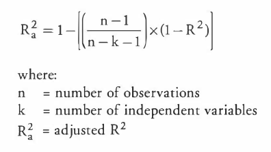
Adjusted R² (RMSE) is the square root of the mean of the squared errors:
Comparing these metrics:
- MAE is the easiest to understand, because it's the average error.
- MSE is more popular than MAE, because MSE "punishes" larger errors, which tends to be useful in the real world.
- RMSE is even more popular than MSE, because RMSE is interpretable in the "y" units.
- R2 the constant baseline is chosen by taking the mean of the data and drawing a line at the mean (always be less than or equal to 1).
- R2 adjusted R² suffers from the problem that the scores improve on increasing terms even though the model is not improving which may misguide the researcher. Adjusted R² is always lower than R² as it adjusts for the increasing predictors and only shows improvement if there is a real improvement.
All of these are loss functions, because we want to minimize them.
from sklearn import metrics
MAE = metrics.mean_absolute_error(y_test, predictions)
MSE = metrics.mean_squared_error(y_test, predictions)
RMSE = np.sqrt(metrics.mean_squared_error(y_test, predictions))

print('MAE:', MAE)
print('MSE:', MSE)
print('RMSE:', RMSE)
print(min(df['y']))
print(max(df['y']))
print(max(df['y']) - min(df['y']))
print('MAE:',MAE/ (max(df['y']) - min(df['y'])))
print('RMSE:',RMSE/(max(df['y']) - min(df['y'])))