Library: Pandas

Installation

Pandas is an open-source library built on top of numpy providing high-performance, easy-to-use data structures and data analysis tools for the Python programming language.
Pandas supports the integration with many file formats or data sources out of the box (csv, excel, sql, json, parquet,…).

In [1]:
#!conda install pandas
#!pip install pandas

import numpy as np
import pandas as pd

Pandas Series

  • One-dimensional ndarray with axis labels, meaning it can be indexed by a label, instead of just a number location.
  • A pandas Series can hold a variety of object types.

Creating Series

(data=None[, index=None, dtype=None, name=None, copy=False, fastpath=False])

In [2]:
labels = ['a','b','c']
my_list = [10,20,30]
arr = np.array([10,20,30])
d = {'a':10,'b':20,'c':30}
In [3]:
#from python list to Series
ser = pd.Series(data=my_list)

ser = pd.Series(data=my_list,index=labels)
ser = pd.Series(my_list,labels)
ser

#from Series to python list
pd.Series.to_list(ser)
Out[3]:
[10, 20, 30]
In [4]:
#from numpy array to Series
ser = pd.Series(arr)
ser = pd.Series(arr,labels)
ser

#from Series to numpy array
pd.Series(ser).array
Out[4]:
<PandasArray>
[10, 20, 30]
Length: 3, dtype: int32
In [5]:
#from python dictionary to Series
ser = pd.Series(d)
ser

#from Series to dictionary
pd.Series.to_dict(ser)
Out[5]:
{'a': 10, 'b': 20, 'c': 30}
In [6]:
ser = pd.Series([10,20,30],['a','b','c'])
ser
Out[6]:
a    10
b    20
c    30
dtype: int64

Indexing and selection

Pandas makes use of these index names or numbers by allowing for fast look ups of information.

In [7]:
ser1 = pd.Series([1,2,3,4],index = ['Enero', 'Febrero','Marzo', 'Abril'])                                   
ser1

ser2 = pd.Series([1,2,5,4],index = ['Enero', 'Febrero','Junio', 'Abril'])
ser2

ser1['Febrero']
ser1.loc['Febrero'] #equivalent, based on label
ser1.iloc[1] #equivalent, based on position
Out[7]:
2

Operations

Based on their associated values.

In [8]:
ser1 + ser2 #NaN when no matching
Out[8]:
Abril      8.0
Enero      2.0
Febrero    4.0
Junio      NaN
Marzo      NaN
dtype: float64
In [9]:
ser1 - ser2 #NaN when no matching
Out[9]:
Abril      0.0
Enero      0.0
Febrero    0.0
Junio      NaN
Marzo      NaN
dtype: float64
In [10]:
ser1 / ser2 #NaN when no matching
Out[10]:
Abril      1.0
Enero      1.0
Febrero    1.0
Junio      NaN
Marzo      NaN
dtype: float64
In [11]:
ser1 * ser2 #NaN when no matching
Out[11]:
Abril      16.0
Enero       1.0
Febrero     4.0
Junio       NaN
Marzo       NaN
dtype: float64

Pandas Data Frames

Two-dimensional, size-mutable, potentially heterogeneous tabular data.

Data structure also contains labeled axes (rows and columns). Arithmetic operations align on both row and column labels. Can be thought of as a dict-like container for Series objects.

Data Input and Output

pandas%20formats.png

Examples

CSV

import

df = pd.read_csv("folder/file.csv")

export

df.to_csv('example',index=False)

EXCEL

import

df = pd.read_excel('file.xlsx', sheet_name='sample')

export

df.to_excel('df.xlsx', sheet_name='sample', index=False)

Creating Data Frames

In [12]:
#passing a dictionaty with columns of different types
df = pd.DataFrame({'A': (1,2,3,4,5,6),
                    'B': pd.Timestamp('20130102'),
                    'C': pd.Series(1, index=list(range(6)), dtype='float32'),
                    'D': np.array([3] * 6, dtype='int32'),
                    'E': pd.Categorical(["test", "train", "test", "train", "test", "train"]), 
                    'F': 'foo'})
df
Out[12]:
A B C D E F
0 1 2013-01-02 1.0 3 test foo
1 2 2013-01-02 1.0 3 train foo
2 3 2013-01-02 1.0 3 test foo
3 4 2013-01-02 1.0 3 train foo
4 5 2013-01-02 1.0 3 test foo
5 6 2013-01-02 1.0 3 train foo

Exploring the DataFrame

In [13]:
df.head(3) #first rows
Out[13]:
A B C D E F
0 1 2013-01-02 1.0 3 test foo
1 2 2013-01-02 1.0 3 train foo
2 3 2013-01-02 1.0 3 test foo
In [14]:
df.tail(3) #last rows
Out[14]:
A B C D E F
3 4 2013-01-02 1.0 3 train foo
4 5 2013-01-02 1.0 3 test foo
5 6 2013-01-02 1.0 3 train foo
In [15]:
df.info() #number of rows, columns, and types
<class 'pandas.core.frame.DataFrame'>
Int64Index: 6 entries, 0 to 5
Data columns (total 6 columns):
 #   Column  Non-Null Count  Dtype         
---  ------  --------------  -----         
 0   A       6 non-null      int64         
 1   B       6 non-null      datetime64[ns]
 2   C       6 non-null      float32       
 3   D       6 non-null      int32         
 4   E       6 non-null      category      
 5   F       6 non-null      object        
dtypes: category(1), datetime64[ns](1), float32(1), int32(1), int64(1), object(1)
memory usage: 342.0+ bytes
In [16]:
df.describe() #basic description of quantitative data
Out[16]:
A C D
count 6.000000 6.0 6.0
mean 3.500000 1.0 3.0
std 1.870829 0.0 0.0
min 1.000000 1.0 3.0
25% 2.250000 1.0 3.0
50% 3.500000 1.0 3.0
75% 4.750000 1.0 3.0
max 6.000000 1.0 3.0
In [17]:
df.dtypes #data type of columns
Out[17]:
A             int64
B    datetime64[ns]
C           float32
D             int32
E          category
F            object
dtype: object
In [18]:
df.columns #column index names
Out[18]:
Index(['A', 'B', 'C', 'D', 'E', 'F'], dtype='object')
In [19]:
del df['F'] #deletes column
df
Out[19]:
A B C D E
0 1 2013-01-02 1.0 3 test
1 2 2013-01-02 1.0 3 train
2 3 2013-01-02 1.0 3 test
3 4 2013-01-02 1.0 3 train
4 5 2013-01-02 1.0 3 test
5 6 2013-01-02 1.0 3 train
In [20]:
df.sort_values(by='A', ascending=False) ##sorting dataframe, inplace=False by default
Out[20]:
A B C D E
5 6 2013-01-02 1.0 3 train
4 5 2013-01-02 1.0 3 test
3 4 2013-01-02 1.0 3 train
2 3 2013-01-02 1.0 3 test
1 2 2013-01-02 1.0 3 train
0 1 2013-01-02 1.0 3 test

Selection and Indexing

In [21]:
from numpy.random import randn
np.random.seed(123)

df = pd.DataFrame(randn(5,4),index='A B C D E'.split(),columns='W X Y Z'.split())
df
Out[21]:
W X Y Z
A -1.085631 0.997345 0.282978 -1.506295
B -0.578600 1.651437 -2.426679 -0.428913
C 1.265936 -0.866740 -0.678886 -0.094709
D 1.491390 -0.638902 -0.443982 -0.434351
E 2.205930 2.186786 1.004054 0.386186
In [22]:
#by row name
df.loc[['B']] #based on label, supports more than one
Out[22]:
W X Y Z
B -0.5786 1.651437 -2.426679 -0.428913
In [23]:
#by row position
df.iloc[[1,2]] #based on position, supports more than one
Out[23]:
W X Y Z
B -0.578600 1.651437 -2.426679 -0.428913
C 1.265936 -0.866740 -0.678886 -0.094709
In [24]:
#by column name
df[['W']]
Out[24]:
W
A -1.085631
B -0.578600
C 1.265936
D 1.491390
E 2.205930
In [25]:
#list of column names
df[['W','Z']]
Out[25]:
W Z
A -1.085631 -1.506295
B -0.578600 -0.428913
C 1.265936 -0.094709
D 1.491390 -0.434351
E 2.205930 0.386186
In [26]:
#by cell, [row,column]
df.loc['B','Y']
Out[26]:
-2.426679243393074
In [27]:
#by group of cell, [rows,columns]
df.loc[['A','B'],['W','Y']]
Out[27]:
W Y
A -1.085631 0.282978
B -0.578600 -2.426679

Conditional selection

In [28]:
#one condition
df[df>0] #NaN = false
Out[28]:
W X Y Z
A NaN 0.997345 0.282978 NaN
B NaN 1.651437 NaN NaN
C 1.265936 NaN NaN NaN
D 1.491390 NaN NaN NaN
E 2.205930 2.186786 1.004054 0.386186
In [29]:
#condition in a column
df[df['W']>0]
Out[29]:
W X Y Z
C 1.265936 -0.866740 -0.678886 -0.094709
D 1.491390 -0.638902 -0.443982 -0.434351
E 2.205930 2.186786 1.004054 0.386186
In [30]:
#condition in a column, select other columns
df[df['W']>0][['Y','X']]
Out[30]:
Y X
C -0.678886 -0.866740
D -0.443982 -0.638902
E 1.004054 2.186786
In [31]:
#two conditions in different columns
df[(df['W']>0) & (df['Y'] > 1)] #being & = AND
Out[31]:
W X Y Z
E 2.20593 2.186786 1.004054 0.386186
In [32]:
#one condition or the other in different columns
df[(df['W']>0) | (df['Y'] > 1)] #being | = OR
Out[32]:
W X Y Z
C 1.265936 -0.866740 -0.678886 -0.094709
D 1.491390 -0.638902 -0.443982 -0.434351
E 2.205930 2.186786 1.004054 0.386186

Modify index

In [33]:
# Reset to default 0,1...n index
df.reset_index()
df
Out[33]:
W X Y Z
A -1.085631 0.997345 0.282978 -1.506295
B -0.578600 1.651437 -2.426679 -0.428913
C 1.265936 -0.866740 -0.678886 -0.094709
D 1.491390 -0.638902 -0.443982 -0.434351
E 2.205930 2.186786 1.004054 0.386186
In [34]:
#new index
nind = 'blue green purple red yellow'.split()
df['Colours'] = nind
df.set_index('Colours')
#df.set_index('Colours',inplace=True) #to make it permanent
df
Out[34]:
W X Y Z Colours
A -1.085631 0.997345 0.282978 -1.506295 blue
B -0.578600 1.651437 -2.426679 -0.428913 green
C 1.265936 -0.866740 -0.678886 -0.094709 purple
D 1.491390 -0.638902 -0.443982 -0.434351 red
E 2.205930 2.186786 1.004054 0.386186 yellow

Creating new column

In [35]:
df['newColumn'] = df['W'] + df['Y']
df
Out[35]:
W X Y Z Colours newColumn
A -1.085631 0.997345 0.282978 -1.506295 blue -0.802652
B -0.578600 1.651437 -2.426679 -0.428913 green -3.005279
C 1.265936 -0.866740 -0.678886 -0.094709 purple 0.587050
D 1.491390 -0.638902 -0.443982 -0.434351 red 1.047408
E 2.205930 2.186786 1.004054 0.386186 yellow 3.209984

Droping column

In [36]:
df.drop('newColumn',axis=1, inplace=True) #inplace=True makes it permanent
df.drop('Colours',axis=1, inplace=True) #inplace=True makes it permanent
df
Out[36]:
W X Y Z
A -1.085631 0.997345 0.282978 -1.506295
B -0.578600 1.651437 -2.426679 -0.428913
C 1.265936 -0.866740 -0.678886 -0.094709
D 1.491390 -0.638902 -0.443982 -0.434351
E 2.205930 2.186786 1.004054 0.386186
In [37]:
df.drop('E',axis=0) #inplace=True makes it permanent
df
Out[37]:
W X Y Z
A -1.085631 0.997345 0.282978 -1.506295
B -0.578600 1.651437 -2.426679 -0.428913
C 1.265936 -0.866740 -0.678886 -0.094709
D 1.491390 -0.638902 -0.443982 -0.434351
E 2.205930 2.186786 1.004054 0.386186

Null values

In [38]:
df = pd.DataFrame({'A':[1,2,np.nan],
                  'B':[5,np.nan,np.nan],
                  'C':[1,2,3]})
df
Out[38]:
A B C
0 1.0 5.0 1
1 2.0 NaN 2
2 NaN NaN 3
In [39]:
df.isnull() #finding nulls
df.isna() #finding na
Out[39]:
A B C
0 False False False
1 False True False
2 True True False
In [40]:
df.dropna() #drops very row with NaN
Out[40]:
A B C
0 1.0 5.0 1
In [41]:
df.dropna(axis=1) #drops every column with NaN
Out[41]:
C
0 1
1 2
2 3
In [42]:
df.dropna(thresh=2) #drops every row with specific number of NaN
Out[42]:
A B C
0 1.0 5.0 1
1 2.0 NaN 2
In [43]:
df.fillna(value='FILL VALUE') #replaces NaN with a defined value
Out[43]:
A B C
0 1 5 1
1 2 FILL VALUE 2
2 FILL VALUE FILL VALUE 3
In [44]:
df['A'].fillna(value=df['A'].mean()) #replaces NaN with the mean of the column
Out[44]:
0    1.0
1    2.0
2    1.5
Name: A, dtype: float64

Multi-Index Hierarchy

In [45]:
#Creates a data frame with multi-index
outside = ['bar', 'bar', 'baz', 'baz', 'foo', 'foo', 'qux', 'qux'] #index generated
inside = ['one', 'two', 'one', 'two', 'one', 'two', 'one', 'two'] #index generated

hier_index = list(zip(outside, inside)) #indexs are zip together
hier_index = pd.MultiIndex.from_tuples(hier_index, names=['first', 'second']) #hierarchy of index applied

df = pd.DataFrame(np.random.randn(8,3), index=hier_index, columns= ['A', 'B', 'C']) #random data generated
df
Out[45]:
A B C
first second
bar one 0.737369 1.490732 -0.935834
two 1.175829 -1.253881 -0.637752
baz one 0.907105 -1.428681 -0.140069
two -0.861755 -0.255619 -2.798589
foo one -1.771533 -0.699877 0.927462
two -0.173636 0.002846 0.688223
qux one -0.879536 0.283627 -0.805367
two -1.727669 -0.390900 0.573806
In [46]:
#change index names
df.index.names
df.index.names = ['first','second']
df
Out[46]:
A B C
first second
bar one 0.737369 1.490732 -0.935834
two 1.175829 -1.253881 -0.637752
baz one 0.907105 -1.428681 -0.140069
two -0.861755 -0.255619 -2.798589
foo one -1.771533 -0.699877 0.927462
two -0.173636 0.002846 0.688223
qux one -0.879536 0.283627 -0.805367
two -1.727669 -0.390900 0.573806
In [47]:
df.loc['foo'] #outer index selected
df.xs('foo') #equivalent
Out[47]:
A B C
second
one -1.771533 -0.699877 0.927462
two -0.173636 0.002846 0.688223
In [48]:
df.loc['foo'].loc['one'] #outer and inner index selected by name
df.xs(['foo','one']) #equivalent
Out[48]:
A   -1.771533
B   -0.699877
C    0.927462
Name: (foo, one), dtype: float64
In [49]:
df.xs('two',level='second') #cross-section function allows indexing directly inner index
Out[49]:
A B C
first
bar 1.175829 -1.253881 -0.637752
baz -0.861755 -0.255619 -2.798589
foo -0.173636 0.002846 0.688223
qux -1.727669 -0.390900 0.573806

Groupby

The groupby method allows to group rows of data together and call aggregate functions.

In [50]:
# Create dataframe
data = {'Company':['GOOG','GOOG','MSFT','MSFT','FB','FB'],
       'Person':['Sam','Charlie','Amy','Vanessa','Carl','Sarah'],
       'Sales':[200,120,340,124,243,350]}
df = pd.DataFrame(data)
df
Out[50]:
Company Person Sales
0 GOOG Sam 200
1 GOOG Charlie 120
2 MSFT Amy 340
3 MSFT Vanessa 124
4 FB Carl 243
5 FB Sarah 350
In [51]:
df.groupby("Company") #group using criteria
df.groupby("Company").mean() #select way of aggregation(ex. mean)
Out[51]:
Sales
Company
FB 296.5
GOOG 160.0
MSFT 232.0
In [52]:
df.groupby("Company").sum() #sum of the group
Out[52]:
Sales
Company
FB 593
GOOG 320
MSFT 464
In [53]:
df.groupby("Company").max() #maximum of the group
Out[53]:
Person Sales
Company
FB Sarah 350
GOOG Sam 200
MSFT Vanessa 340
In [54]:
df.groupby("Company").std() #standard deviation of the group
Out[54]:
Sales
Company
FB 75.660426
GOOG 56.568542
MSFT 152.735065
In [55]:
df.groupby("Company").count() #count cases of the group
Out[55]:
Person Sales
Company
FB 2 2
GOOG 2 2
MSFT 2 2
In [56]:
df.groupby("Company").describe().transpose() #describe + transpose
Out[56]:
Company FB GOOG MSFT
Sales count 2.000000 2.000000 2.000000
mean 296.500000 160.000000 232.000000
std 75.660426 56.568542 152.735065
min 243.000000 120.000000 124.000000
25% 269.750000 140.000000 178.000000
50% 296.500000 160.000000 232.000000
75% 323.250000 180.000000 286.000000
max 350.000000 200.000000 340.000000

Merging, Joining, and Concatenating

In [57]:
df1 = pd.DataFrame({'A': ['A0', 'A1', 'A2', 'A3'],
                    'B': ['B0', 'B1', 'B2', 'B3'],
                    'C': ['C0', 'C1', 'C2', 'C3'],
                    'D': ['D0', 'D1', 'D2', 'D3']},
                    index=[0, 1, 2, 3])
df1
Out[57]:
A B C D
0 A0 B0 C0 D0
1 A1 B1 C1 D1
2 A2 B2 C2 D2
3 A3 B3 C3 D3
In [58]:
df2 = pd.DataFrame({'A': ['A4', 'A5', 'A6', 'A7'],
                    'B': ['B4', 'B5', 'B6', 'B7'],
                    'C': ['C4', 'C5', 'C6', 'C7'],
                    'D': ['D4', 'D5', 'D6', 'D7']},
                    index=[4, 5, 6, 7])
df2
Out[58]:
A B C D
4 A4 B4 C4 D4
5 A5 B5 C5 D5
6 A6 B6 C6 D6
7 A7 B7 C7 D7

Concatenate

Dimensions should match along the axis you are concatenating on, gets all the rows together.

In [59]:
pd.concat([df1,df2], axis=0, join='outer', ignore_index=False, keys=None,
          levels=None, names=None, verify_integrity=False, copy=True)
Out[59]:
A B C D
0 A0 B0 C0 D0
1 A1 B1 C1 D1
2 A2 B2 C2 D2
3 A3 B3 C3 D3
4 A4 B4 C4 D4
5 A5 B5 C5 D5
6 A6 B6 C6 D6
7 A7 B7 C7 D7
In [60]:
result = df1.append(df2) #equivalent
result
Out[60]:
A B C D
0 A0 B0 C0 D0
1 A1 B1 C1 D1
2 A2 B2 C2 D2
3 A3 B3 C3 D3
4 A4 B4 C4 D4
5 A5 B5 C5 D5
6 A6 B6 C6 D6
7 A7 B7 C7 D7

Merge

Allows you to merge DataFrames together using a similar logic as merging SQL Tables together.

In [61]:
#creates left table
left = pd.DataFrame({'key': ['K0', 'K1', 'K2', 'K3'],
                     'A': ['A0', 'A1', 'A2', 'A3'],
                     'B': ['B0', 'B1', 'B2', 'B3']})
left

#creates right table
right = pd.DataFrame({'key': ['K0', 'K1', 'K2', 'K3'],
                          'C': ['C0', 'C1', 'C2', 'C3'],
                          'D': ['D0', 'D1', 'D2', 'D3']})
right

#performs INNER merge (only coincidences in key between dataframes are kept)
pd.merge(left, right, how='inner', on='key', left_on=None, right_on=None,
         left_index=False, right_index=False, sort=True,
         suffixes=('_x', '_y'), copy=True, indicator=False,
         validate=None)
Out[61]:
key A B C D
0 K0 A0 B0 C0 D0
1 K1 A1 B1 C1 D1
2 K2 A2 B2 C2 D2
3 K3 A3 B3 C3 D3
In [62]:
#creates left table
left = pd.DataFrame({'key1': ['K0', 'K0', 'K1', 'K2'],
                     'key2': ['K0', 'K1', 'K0', 'K1'],
                        'A': ['A0', 'A1', 'A2', 'A3'],
                        'B': ['B0', 'B1', 'B2', 'B3']})

#creates left table
right = pd.DataFrame({'key1': ['K0', 'K1', 'K1', 'K2'],
                        'key2': ['K0', 'K0', 'K0', 'K0'],
                        'C': ['C0', 'C1', 'C2', 'C3'],
                        'D': ['D0', 'D1', 'D2', 'D3']})

#performs inner merge (only coincidences between dataframes in both keys are kept)
pd.merge(left, right, on=['key1', 'key2'])
Out[62]:
key1 key2 A B C D
0 K0 K0 A0 B0 C0 D0
1 K1 K0 A2 B2 C1 D1
2 K1 K0 A2 B2 C2 D2
In [63]:
#performs OUTER merge (all cases are kept)
pd.merge(left, right, how='outer', on=['key1', 'key2'])
Out[63]:
key1 key2 A B C D
0 K0 K0 A0 B0 C0 D0
1 K0 K1 A1 B1 NaN NaN
2 K1 K0 A2 B2 C1 D1
3 K1 K0 A2 B2 C2 D2
4 K2 K1 A3 B3 NaN NaN
5 K2 K0 NaN NaN C3 D3
In [64]:
#performs RIGHT merge (all cases of right dataframe are kept)
pd.merge(left, right, how='right', on=['key1', 'key2'])
Out[64]:
key1 key2 A B C D
0 K0 K0 A0 B0 C0 D0
1 K1 K0 A2 B2 C1 D1
2 K1 K0 A2 B2 C2 D2
3 K2 K0 NaN NaN C3 D3
In [65]:
#performs LEFT merge (all cases of left dataframe are kept)
pd.merge(left, right, how='left', on=['key1', 'key2'])
Out[65]:
key1 key2 A B C D
0 K0 K0 A0 B0 C0 D0
1 K0 K1 A1 B1 NaN NaN
2 K1 K0 A2 B2 C1 D1
3 K1 K0 A2 B2 C2 D2
4 K2 K1 A3 B3 NaN NaN

Join

Combining the columns of two potentially differently-indexed DataFrames into a single result DataFrame.

In [66]:
left = pd.DataFrame({'A': ['A0', 'A1', 'A2'],
                     'B': ['B0', 'B1', 'B2']},
                      index=['K0', 'K1', 'K2']) 

right = pd.DataFrame({'C': ['C0', 'C2', 'C3'],
                    'D': ['D0', 'D2', 'D3']},
                      index=['K0', 'K2', 'K3'])
left.join(right) #inner join
Out[66]:
A B C D
K0 A0 B0 C0 D0
K1 A1 B1 NaN NaN
K2 A2 B2 C2 D2
In [67]:
left.join(right, how='outer') #outer join
Out[67]:
A B C D
K0 A0 B0 C0 D0
K1 A1 B1 NaN NaN
K2 A2 B2 C2 D2
K3 NaN NaN C3 D3

Operations

In [68]:
#creates data frame
df = pd.DataFrame({'col1':[1,2,3,4],'col2':[444,555,666,444],'col3':['abc','def','ghi','xyz']})
df
Out[68]:
col1 col2 col3
0 1 444 abc
1 2 555 def
2 3 666 ghi
3 4 444 xyz
In [69]:
#Select from DataFrame using criteria from multiple columns
newdf = df[(df['col1']>2) & (df['col2']==444)]
newdf
Out[69]:
col1 col2 col3
3 4 444 xyz
In [70]:
#list of unique values
df['col2'].unique()
Out[70]:
array([444, 555, 666], dtype=int64)
In [71]:
#number of unique values
df['col2'].nunique() 
Out[71]:
3
In [72]:
#amount of each value
df['col2'].value_counts() 
Out[72]:
444    2
555    1
666    1
Name: col2, dtype: int64
In [73]:
#Applying created functions
def times2(x):
    return x*2

df['col1'].apply(times2)
Out[73]:
0    2
1    4
2    6
3    8
Name: col1, dtype: int64
In [74]:
#Applying standard functions
df['col3'].apply(len) #lenght of the values
df['col1'].sum() #sum of the values
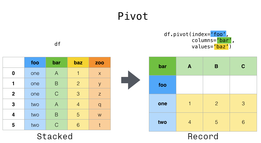
Out[74]:
10

Pivot table

pivot

In [75]:
#creates data frame from dictionary
data = {'A':['foo','foo','foo','bar','bar','bar'],
     'B':['one','one','two','two','one','one'],
       'C':['x','y','x','y','x','y'],
       'D':[1,3,2,5,4,1]}
df = pd.DataFrame(data)
df
Out[75]:
A B C D
0 foo one x 1
1 foo one y 3
2 foo two x 2
3 bar two y 5
4 bar one x 4
5 bar one y 1
In [76]:
#creates pivot table
df.pivot_table(values='D',index=['A', 'B'],columns=['C'])
Out[76]:
C x y
A B
bar one 4.0 1.0
two NaN 5.0
foo one 1.0 3.0
two 2.0 NaN

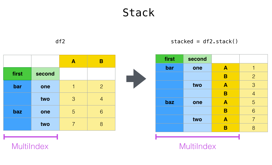
Reshaping by stacking

stack

In [77]:
df
Out[77]:
A B C D
0 foo one x 1
1 foo one y 3
2 foo two x 2
3 bar two y 5
4 bar one x 4
5 bar one y 1
In [78]:
df2 = df[:4]
df2
Out[78]:
A B C D
0 foo one x 1
1 foo one y 3
2 foo two x 2
3 bar two y 5
In [79]:
#Stacking
stacked = df2.stack()
dfstacked = pd.DataFrame(stacked, columns =['cases'])
dfstacked
Out[79]:
cases
0 A foo
B one
C x
D 1
1 A foo
B one
C y
D 3
2 A foo
B two
C x
D 2
3 A bar
B two
C y
D 5
In [80]:
#Unstacking
dfstacked.unstack()
Out[80]:
cases
A B C D
0 foo one x 1
1 foo one y 3
2 foo two x 2
3 bar two y 5

Reshaping by Melt

Melt

In [81]:
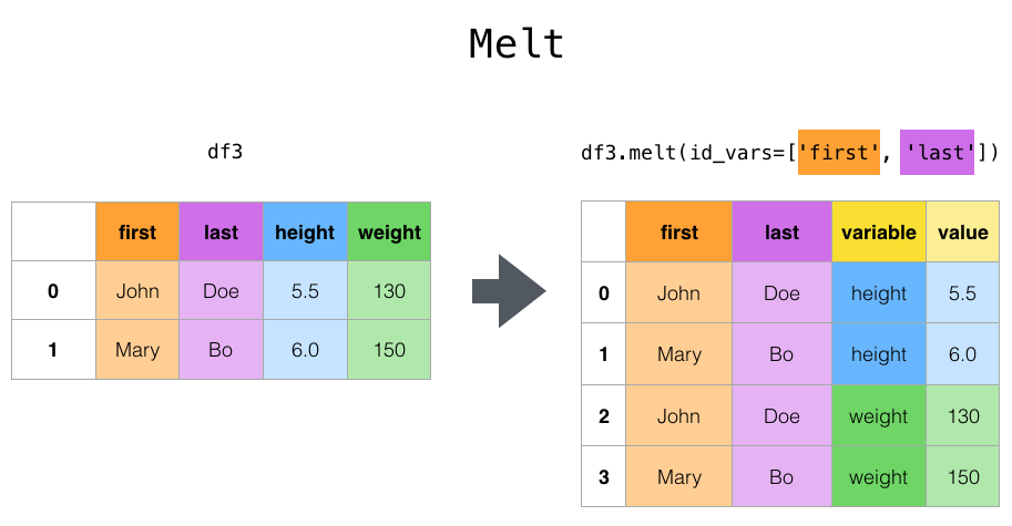
cheese = pd.DataFrame({'first': ['John', 'Mary'],
                       'last': ['Doe', 'Bo'],
                       'height': [5.5, 6.0],
                       'weight': [130, 150]})
cheese
Out[81]:
first last height weight
0 John Doe 5.5 130
1 Mary Bo 6.0 150
In [82]:
cheese.melt(id_vars=['first', 'last'], var_name='quantity')
Out[82]:
first last quantity value
0 John Doe height 5.5
1 Mary Bo height 6.0
2 John Doe weight 130.0
3 Mary Bo weight 150.0

Data visualization

In [83]:
import matplotlib as plt
import seaborn as sns

# loading databases
tips = sns.load_dataset('tips')
tips.head()
Out[83]:
total_bill tip sex smoker day time size
0 16.99 1.01 Female No Sun Dinner 2
1 10.34 1.66 Male No Sun Dinner 3
2 21.01 3.50 Male No Sun Dinner 3
3 23.68 3.31 Male No Sun Dinner 2
4 24.59 3.61 Female No Sun Dinner 4
In [84]:
%matplotlib inline

Styles

In [85]:
#set matplotlib style
plt.style.use('default')
tips['total_bill'].hist()
Out[85]:
<matplotlib.axes._subplots.AxesSubplot at 0x1a2ec328508>
In [86]:
plt.style.use('ggplot')
tips['total_bill'].hist()
Out[86]:
<matplotlib.axes._subplots.AxesSubplot at 0x1a2ecbe0b48>
In [87]:
plt.style.use('bmh')
tips['total_bill'].hist()
Out[87]:
<matplotlib.axes._subplots.AxesSubplot at 0x1a2ecafed88>
In [88]:
plt.style.use('fivethirtyeight')
tips['total_bill'].hist()
Out[88]:
<matplotlib.axes._subplots.AxesSubplot at 0x1a2eadb7088>
In [89]:
plt.style.use('classic')
tips['total_bill'].hist()
Out[89]:
<matplotlib.axes._subplots.AxesSubplot at 0x1a2ecc32c88>
In [90]:
plt.style.use('grayscale')
tips['total_bill'].hist()
Out[90]:
<matplotlib.axes._subplots.AxesSubplot at 0x1a2ecccf1c8>
In [91]:
plt.style.use('seaborn')
tips['total_bill'].hist()
Out[91]:
<matplotlib.axes._subplots.AxesSubplot at 0x1a2eccd6d48>

Graphic types

In [92]:
df1 = tips[0:20][['total_bill', 'tip']]
df1.head()

df2 = tips[['total_bill', 'tip', 'day']]
df2.head()

df3 = tips[0:20][['total_bill', 'tip', 'size']]
df3.head()
Out[92]:
total_bill tip size
0 16.99 1.01 2
1 10.34 1.66 3
2 21.01 3.50 3
3 23.68 3.31 2
4 24.59 3.61 4
In [93]:
df1.plot.area() #can only use quantitative information, qualitative make error
Out[93]:
<matplotlib.axes._subplots.AxesSubplot at 0x1a2ecde2b08>
In [94]:
df1.plot.barh(stacked=True) #can only work with quantitative data, skips qualitative
Out[94]:
<matplotlib.axes._subplots.AxesSubplot at 0x1a2ece76648>
In [95]:
df1.plot.density() #distribution of quantitative data, skips qualitative
Out[95]:
<matplotlib.axes._subplots.AxesSubplot at 0x1a2ed1f85c8>
In [96]:
df2['total_bill'].plot.hist(bins = 10) #distribution of quantitative data, skips qualitative
Out[96]:
<matplotlib.axes._subplots.AxesSubplot at 0x1a2ed117788>
In [97]:
df2.plot.line(figsize=(12,3),lw=1) #works with quantitative data, skips qualitative
Out[97]:
<matplotlib.axes._subplots.AxesSubplot at 0x1a2ed19c288>
In [98]:
df3.plot.scatter(x = 'total_bill', y = 'tip', c = 'size', s=df3['size']*100, cmap = 'rainbow') #can only use quantitative information, qualitative make error
Out[98]:
<matplotlib.axes._subplots.AxesSubplot at 0x1a2ee244408>
In [99]:
df1.plot.bar(stacked = True) #can only work with quantitative data, skips qualitative
Out[99]:
<matplotlib.axes._subplots.AxesSubplot at 0x1a2ee442b48>
In [100]:
df1.plot.box() #categories are the columns, can be used "by = " for groupby
Out[100]:
<matplotlib.axes._subplots.AxesSubplot at 0x1a2ee3e47c8>
In [101]:
df1.plot.hexbin('total_bill', 'tip',gridsize=25,cmap='Blues') #distribution of quantitative data, skips qualitative
Out[101]:
<matplotlib.axes._subplots.AxesSubplot at 0x1a2ee4e0f88>
In [102]:
df1.plot.kde()
Out[102]:
<matplotlib.axes._subplots.AxesSubplot at 0x1a2ee6d61c8>